SIL Calcs 101: Intro
Introductory post in the SIL Calcs 101 series.
Welcome! This series of posts will attempt to demystify safety integrity level calculations (SIL Calcs). The idea is to teach you how to do these calculations in an intuitive, and illustrative way, so that you can wrap your head around what is actually going on. We’ll be using a simple approach, simple enough to model in Excel. Note, however, that we will not be using the simplified equations (as commonly used when computing by hand).
Our approach will be a little different than what the commercial SIL solver applications use—they tend to use Markov models, which I may cover in a future post. The reasoning behind our approach is threefold: its plenty accurate for learning purposes (please do actual SIL calcs with validated software), is a perfectly valid method, and it’s way more intuitive than other methods. With that, let’s just get to it.
Safety Instrumented Systems: PFD Average
So you’ve got yourself a new (or are supporting an old) safety instrumented system (SIS), and you need to do some SIL calcs. First thing is first: what are we actually calculating when we do a SIL calc?
Might seem like a simple question, but it’s terribly important. When doing the calcs for a low demand system, we are trying to calculate the PFD (probability of failure on demand) average for the system (over some fixed time period—commonly referred to as the mission time). I am going to represent this quantity like so:
Just keep in mind that this is the thing we are looking for. It’s an average over some fixed timeframe.
We’ve established that we are looking for the average value of a thing, this implies that we need some kind of information about the thing itself. For example, if I wanted to find the average age of all the people in the room, it would help to know the ages of all the people in the room! Clearly, to compute the PFD average, we need to know how to compute the PFD (probability of failure on demand).
Safety Integrity Level Calculation: Basic Equation
Presented below is an equation for PFD of a single element system. It’s possible to derive this, but we’ll do that another time. For now, let’s just take it as a well established equation:
Where PFD is the probability of failure on demand at some time t, and lambda is our failure rate (dangerous undetected failures).
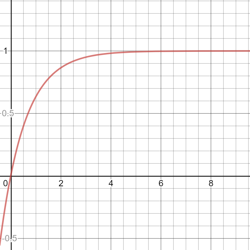
I would be remiss if I didn’t include a basic plot of this function. Below it’s plotted with lambda = 1 for simplicity. Note that the y-axis is PFD, and the x-axis is time (since lambda is 1 the units on time aren’t terribly important here, call it years for now):
It’s important to understand that lambda is just a number, and so the variable in this equation is time. I.e. this is just a function of time.
A Math Problem
Really then, what we are trying to do is find the average of this function over some specific time interval (the mission time of our SIF). Well, this is just a math problem! You may question my excitement here, but I maintain that anytime we take our engineering problem, and successfully reduce it to a well defined math problem, we’re doing alright.
So what exactly is our well defined math problem? Said in words, we are trying to find the average value of a function over a fixed time interval. If we can do that, then we have our PFD average, which means we can determine our SIL level from the IEC 61508 tables, and we are done with our calc.
There are two main approaches to solving this problem: analytical and numerical. We will be covering the latter in this series, though at some point I will post about the analytical solution. Our reasons for choosing the numerical approach are:
- The analytical approach becomes prohibitively difficult as the system complexity grows
- The numerical solution is plenty accurate
- Industry standard practice is to use numerical approximation
In the remainder of this series I am going to show you how to numerically approximate the PFD for a single element system, and then to use that as a building block for more complex systems.
I think we have covered sufficient ground for our introductory post. Next time we’ll dive straight into the details of modeling the single element system.