SIL Calcs 101: Single Element System
A simple system example.
Alright, lets have some fun. We are going to model a single element (1oo1) system. Recall our basic equation from last time.
Let’s model a level switch. First, we’ll need failure rate data (so that we know what lambda is). For simplicity, we will just take the high bound dangerous failure rate from http://silsafedata.com/. Scroll down the website until you see “Level Switch”, with DU high bound of 1000. The units on this number are FITs or failures per billion hours. Let’s convert that to failures per hour real quick:
Safety Integrity Level Spreadsheet Permalink
Open your favorite spreadsheet app, and enter the info for our lambda, like so:
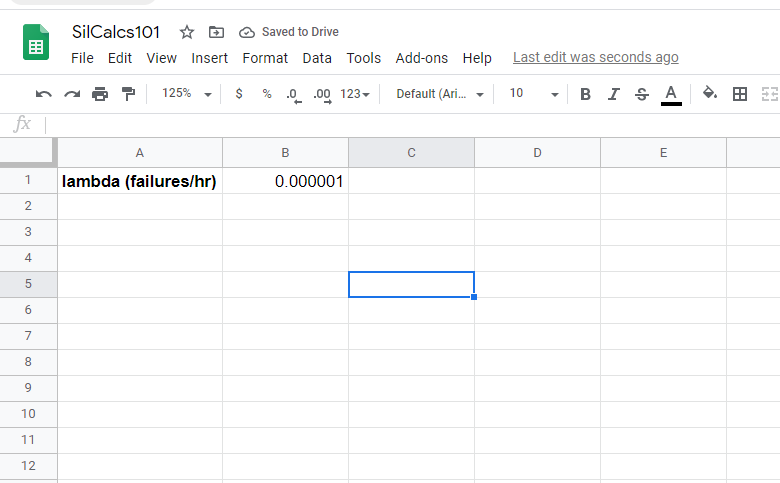
You can find my sheet at: spreadsheet
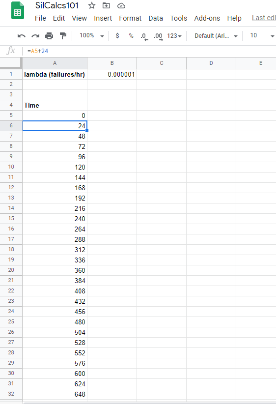
Now we need to pick a time step. Time is the independent variable in our equation for PFD. In order to approximate this function, we need to evaluate it at a bunch of different points in time! For simplicity, let’s evaluate the function on a daily basis (i.e every 24 hours). We also need to define the mission time (aka the timeframe over which we are finding the average PFD). Let’s use 1 year, this keeps us from having way too many rows in our spreadsheet.
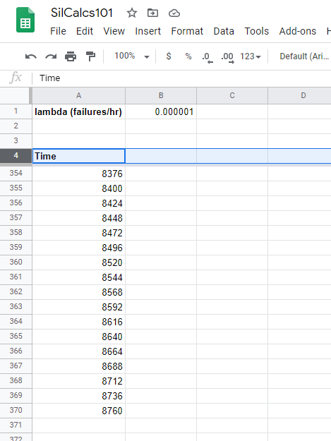
Recall that 1 year = 365 days * 24 hrs/day = 8760 hrs
Note that the units of your timestep and your failure rate need to match. We will do both in hours.
So, if you are following along, build out the time step column like so:
Your “time” column should continue to 8760 hours:
Once that’s complete, it’s time to model the PFD of our level switch. Remember this is a single element, one out of one (1oo1) system.
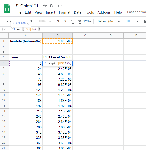
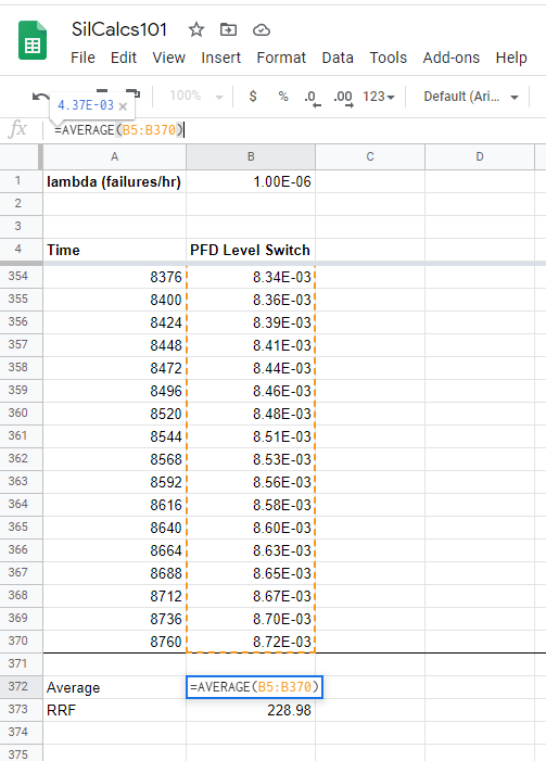
We have a value for lambda (from SILsafe data), we have a time column all ready to go, now all we need to do is model the system by entering our formula for PFD into the sheet, and using the time column as the independent variable in the equation. See my sheet below if your are confused, note the contents of my formula bar:
Watch out for those dollar signs around the value of lambda! It needs to remain constant over the entire time frame (this is technically known as the constant failure rate assumption, possibly a blog for another day).
Fill this formula all the way down. At the bottom, compute the average of the system. Also shown in my sheet is the risk reduction factor (RRF), which is just the inverse of PFD average (1/PFD average).
And there you have it, you’ve just successfully computed the PFD average for a 1oo1 system. Our result is, for a mission time of 1 year:
We’ll talk in detail about how to extend this to more complex systems, and eventually entire safety instrumented functions (SIFs) in the next post. For now, let’s graph this and make sure it looks alright.
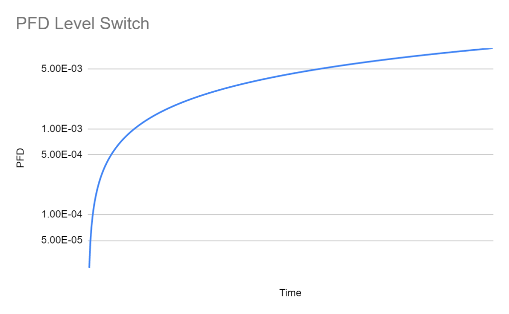
Looks good to me. Note that I am using a log scale on the vertical axis here.
See you in the next post.