SIL Calcs 101: Proof Testing

Posted in SIL Calcs 101 on Proof Testing

Proof Testing Basics.

Time to complicate our lives a bit! Proof testing is essential to most safety integrity level calculations, and while the details of how to calculate proof test coverages, or how to execute good proof tests, are worthwhile topics, this post is going to focus on the nuts and bolts of modeling proof testing.

Proof Test Example

The best way to do this is to just dive straight into an example. It’s worth noting that we are going to do this the long way the first time through, after which we will generalize and also automate the method a bit.

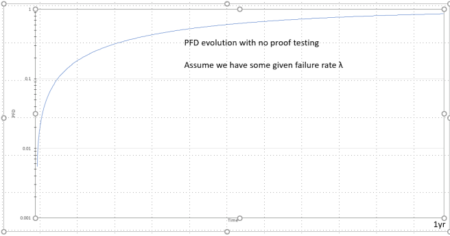
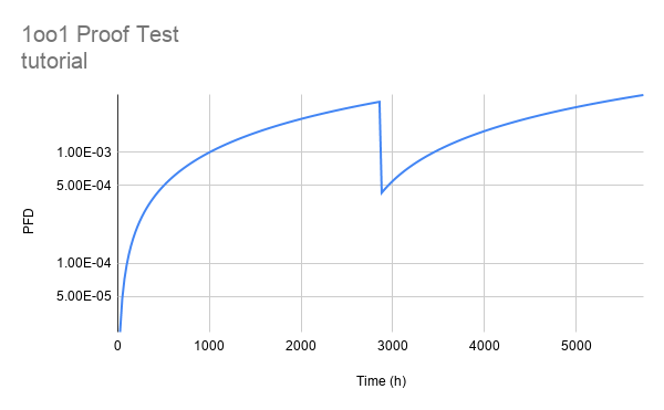
Look at the first graph below, it shows the evolution of a single element system with no proof testing. Assume that the system has some lambda value, it doesn’t much matter what it is for right now.

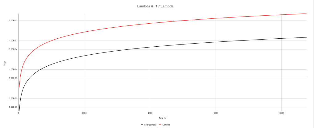
Now check out the next graph, it still has the system above, but I have added a system that has 15% of the lambda of the original system. We’ll talk more about what this means later, but for now, consider it a useful reference when thinking about proof testing.

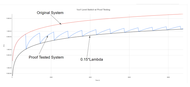
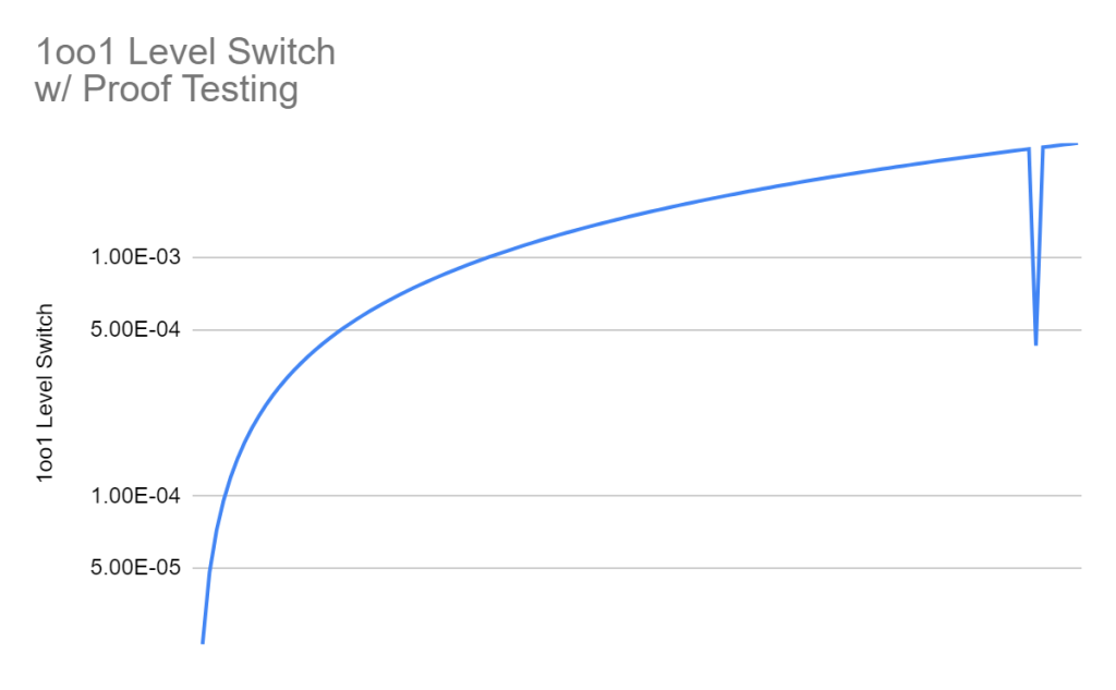
The next graph shows the evolution of a proof tested system superimposed over the original non-proof tested system (with the 15% lambda system on the graph as a reference). The two superimposed systems (proof tested and not proof tested) have the same lambda. The proof test is done with 85% coverage, which we will talk about in just a minute.

If you are unfamiliar with the notion of proof testing, those sudden vertical drops in PFD are where we are executing the proof tests. Testing is typically done at regular intervals; we go out to the field and stroke the valve, float the level switch, etc. The test either proves that the system is functional, or finds defects that need to be repaired.

Based on the completeness/rigor of the test, we take a certain amount of credit, e.g. we might take 85% credit for stroking a valve. What this says is that we are confident that, with the testing done, we’ve found 85% of the possible failures for that valve. This implies that 15% of the failures could not be found by our test, and so we drop the PFD of our system down so that it meets up with the PFD of a system with only 15% of the lambda value.

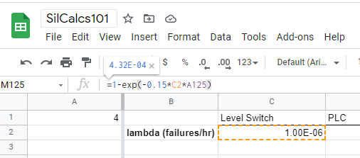
What’s really important to notice here is that the proof tested system is exactly the same as the untested system, up until the point of the first proof test. The two systems literally sit on top of each other in the graph. With that in mind, lets start modeling our proof tested system. We’ll stick with a 1oo1 system for now, go ahead and add a column to your spreadsheet for this model:

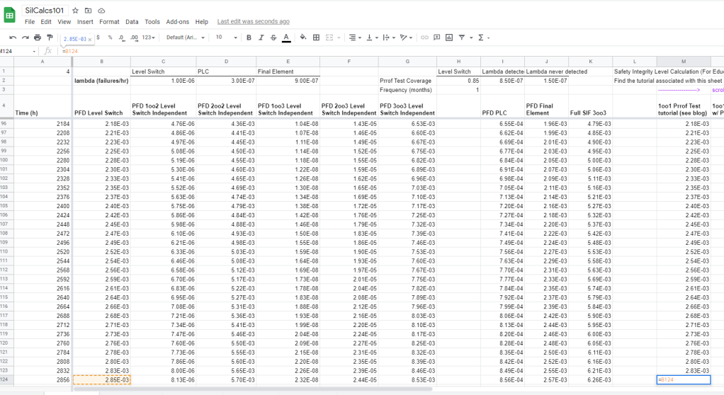
Notice that I just set the PFD (probability of failure on demand) equal to the basic, single level switch, case. Again, this is because, until we actually go out and do a proof test, the system is identical to the untested case. Also notice that I modeled down to time 2856 hours. We are going to do our proof tests at four month intervals: 30 days in a month x 24 hours in a day x 4 months = 2880 hours. So, hour 2856 is the day before the proof test! Basically, we’ve modeled up until the point where we execute the test, now we need to talk about what happens on the day of the proof test.

We go out and do the test, and either we prove that everything works, or we find issues and correct them. Assume that our proof test has 85% coverage, that means that we find 85% of the potential failures of our level switch. We model this by adjusting our probability of failure on demand down, specifically we drop the PFD down to the level of a system with 15% of the lambda:

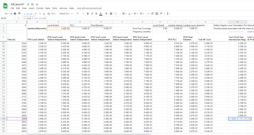
Notice that I calculate the PFD on the day of the proof test by evaluating a system with 0.15*λ. Why is this justified? Well, we’ve found all of the failures—via our proof test—associated with 85% of the level switch’s lambda (i.e I went out and float tested the level switch, and on the basis of that test, I am confident that of all the possible ways the level switch could be failed, 85% of them can’t possibly be true) so, the failures that are left must correspond to the 15% of lambda we were unable to test. These failures grow unfettered since the moment the device is put into service, so on the day of the proof test, it’s reasonable to say that the PFD of the level switch, after testing, is simply the PFD associated with the 15% of failures we couldn’t find.

After the Proof Test

Great, we did a proof test, and even better, we modeled it! What now? The key question here is, how does the system evolve in time after we do the proof test. Well, it evolves the same as before, according to the basic equation, and governed by lambda. What, however, would you propose we input for time in our equation? Think about this for a minute, if we just carry on, plugging in the next day—hour 2904—what would our system look like? Let me graph that approach for you:

This can’t be right. We went out and did a proof test, our PFD dropped for a second, and then shot right back up to where it was before. Remember that this is a model, not reality. Out in the field time moves ahead as normal, but we are modeling PFD using the equation: $$\begin{equation} PFD=1-e^{-\lambda t} \end{equation}$$

This is a straightforward function of time: it maps values of PFD to unique values of time. So, if our PFD after the proof test is lower, then we can conclude that our time must be earlier!

What this is telling us is that after we proof test, our level switch is acting like a newer version of itself. This should strike you as reasonable, after all, we did just go out and prove that a bunch of failures didn’t exist. If this is confusing you, remember that we are speaking in terms of our model here. The level switch out in the field is four months old, but we’ve proved that our switch has a lower PFD than we originally anticipated, so mathematically speaking, it is behaving like a younger switch.

If this notion still doesn’t resonate with you, it’s alright. It’s just my intuitive way of understanding what is going on. It’s good enough if you just realize that the level switch’s PFD dropped, and so we need to compute the time that matches up with that lower PFD.

Calculating Time from PFD

How then, do we compute the time that goes with our lower PFD after proof testing? Take a look at the basic equation again: $$\begin{equation} PFD=1-e^{-\lambda t} \end{equation}$$

All we need to do is solve this for time. Let’s just do it: $$\begin{equation} e^{-\lambda t} = 1 - PFD \end{equation}$$ $$\begin{equation} -\lambda t = ln(1 - PFD) \end{equation}$$ $$\begin{equation} t = \frac{-ln(1-PFD)}{\lambda} \end{equation}$$

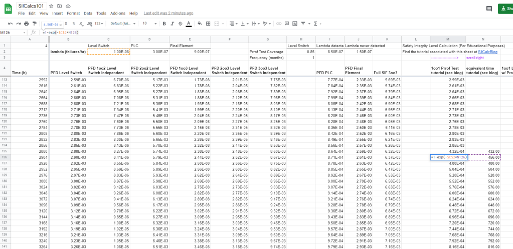
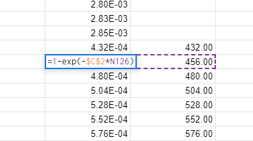
Start a new column in the spreadsheet, use it as a place to calculate our “equivalent time”. Use the formula above for the calculation:

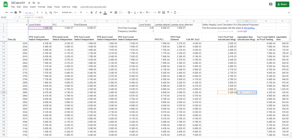
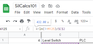
I calculate that our proof tested PFD corresponds to a time of 432 hours. From here, continue stepping forward in time by 24 hour increments:

Carry this forward until the day before the next proof test, which occurs at the eight month mark (5760 hours is eight months).

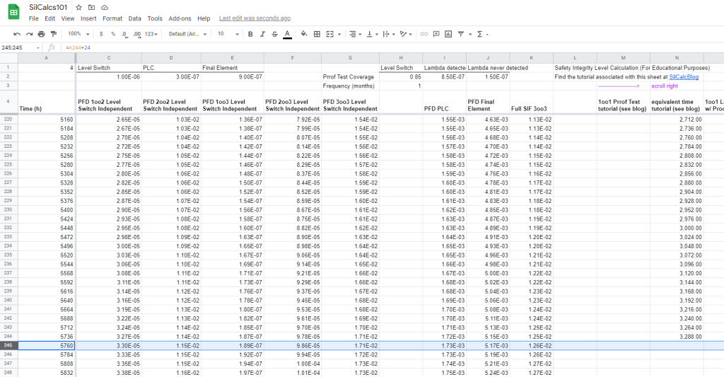
Now, as discussed above, we know the system evolves according to the basic equation between proof tests. Just remember that we need to model using the equivalent time:

As always, mind those dollar signs around your lambda! Model the PFD down to the day before the eight month proof test. Let’s check the graph to see how we are looking:

Looking good.

Modeling the Remaining Tests

At this point we just repeat the process again at the eight month mark, and at the twelve month mark. Once again, we drop PFD to meet up with the 15% lambda system. Then we calculate equivalent time, and we step forward in 24 hour increments from there. The PFD of the system gets modeled based on the equivalent time. Don’t forget to compute PFD average and RRF when you are done, the details are all in the spreadsheet. Let’s check the graph:

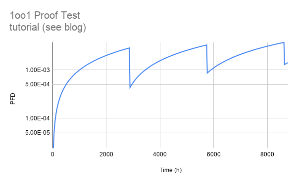
Excellent stuff!

Generalizing and Automating

I don’t know about you, but I do not want to sit and go through that tedious process every time I want to model a proof test, change a proof test frequency, or change a proof test coverage. We need some automation here.

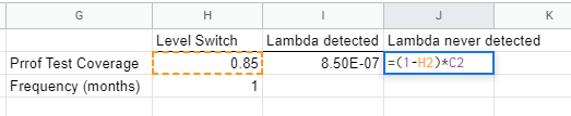
First, let’s define some parameters we need, namely the proof test coverage and frequency:

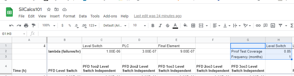
Every time we go proof test our device (at whatever frequency) we know we are going to drop PFD down to the 15% lambda system. More generally, we drop down to a system with lambda = 1 – proof test coverage: $$\begin{equation} \lambda_{ND} = (1-PTC)\lambda_{DU} \end{equation}$$

Where λ_ND stands for “lambda never detected”, λ_DU is just our level switch’s original value of lambda, and PTC stands for “proof test coverage”.

Go ahead and compute λ_ND, and while you are at it, compute lambda detected (via the proof test) as: $$\begin{equation} \lambda_{DD} = \lambda_{DU}*PTC \end{equation}$$

Where λ_DD is lambda detected.

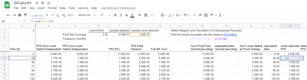
Next, model the λ_ND system over our entire timeframe, that way whenever we need to know what it’s value is, we have it handy:

Building Some Logic

Think through what we want to do: if it’s the day of a proof test (based on our proof test frequency), then we want the PFD of the system to fall to the λND system, otherwise, we want the system to evolve in time normally. How to tell if it’s the day of a proof test? Use the modulo operation! The modulo operation returns the remainder of a division, for example: 5mod2 evaluates to 1, since the remainder when you divide 5 by 2 is 1. Similarly, 9mod3 evaluates to zero.

Consider a proof test frequency of 720 hours (1 month). Try working through a couple of examples (note these all have units of hours):

24mod720 = 24

48mod720 = 48

720mod720 = 0

744mod720 = 24

768mod720 = 48

1440mod720 = 0

1464mod720 = 24

The key insight here is that the modulo operation evaluates to 0 when the numbers cleanly divide; we can use this to our advantage: if the current time modulo proof test frequency = 0, then it’s time for a proof test! Otherwise, evolve normally in time.

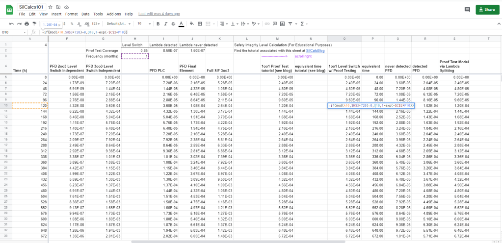
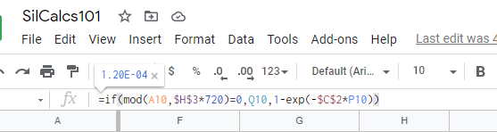
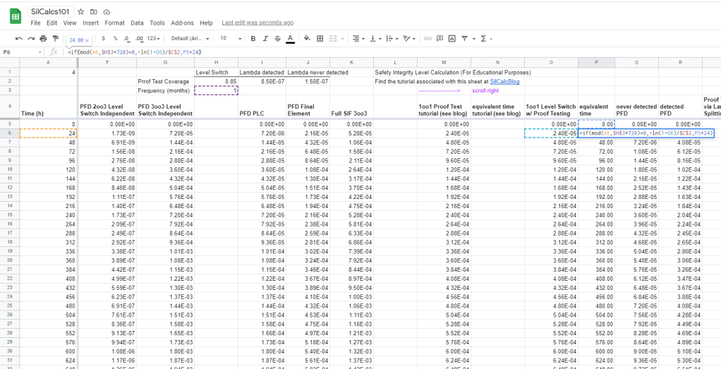
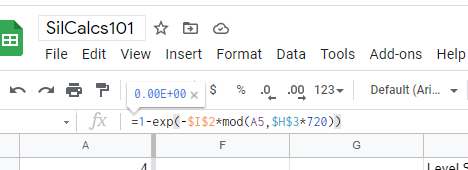
This is exactly what we wanted, if cell A10 (current time) modulo proof test frequency (notice I converted to hours by multiplying by 720 hours/month) equals zero, then we set the PFD equal to Q10 (which is the PFD of the never detected system). Otherwise, we compute PFD as normal. Notice that we still use cell C2 as the lambda, because the system evolves in time according to its overall failure rate, unless we are doing something to it, like proof testing it. Also note that instead of time (column A) I used equivalent time here (column P). More on that in a minute.

Fill this formula in all the way down, and now lets talk time.

Equivalent Time, Automated

Again, think through what it is we are trying to do: when it’s time for a proof test, we want to calculate the equivalent time via: $$\begin{equation} t = \frac{-ln(1 - PFD)}{\lambda} \end{equation}$$

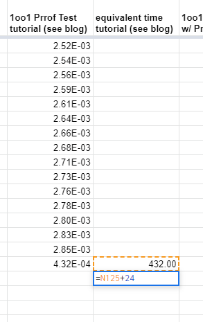
When it’s not time for a proof test, we want to add 24 hours to whatever the previous time was. The modulo operation works quite well here, this is basically the same logic as we used for the PFD column.

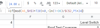
All we are doing here is checking if it’s proof test time (via modulo operation), if it is we calculate the equivalent time, else we add 24 hours to the previous time. Note that we need to enter 0 hours manually into the first cell (because there is nothing above it to add 24 hours to):

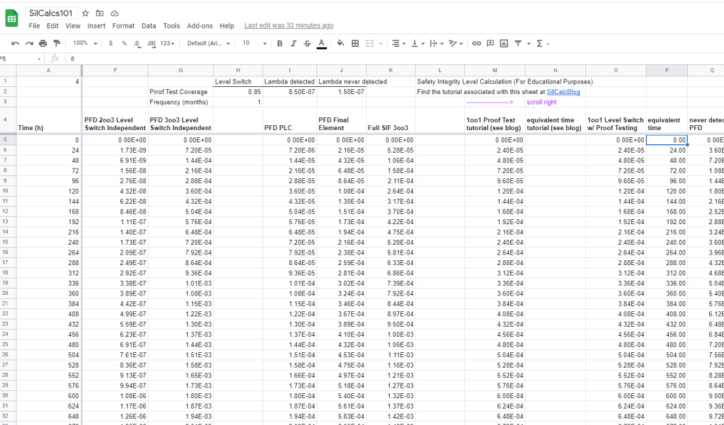
That’s all there is to it, with this simple logic the proof testing calculations are automated, all you need to do is adjust your frequency and coverage as desired. Note that since our timestep here is 24 hours, using a proof test frequency that isn’t an integer multiple of 24 will likely produce unexpected results.

Lambda Splitting

Formal contexts, such as a textbook, won’t use the method we’ve outlined above. Instead, you will see an entirely equivalent method, based around the idea of splitting lambda up into two pieces. We have already seen both of these pieces, they are λ_ND and λ_DD, which we computed above. Last time we didn’t do much of anything with λ_DD, but this time it will play a central role.

The approach of the lambda splitting method is to model each piece of lambda as it’s own system, and then to join them. The lambda never detected system is easy to model, in fact, we’ve already done it above. The lambda detected system requires an extra second of thought; what we want to do here is model a system that evolves in time normally, until there is a proof test, at which point all of the failures are found. Why? Because the lambda detected system is the set of all failures which are detected by our (imperfect) proof test. Basically, we need to model the lambda detected system with 100% proof test coverage, which we already know how to do, so let’s get to it.

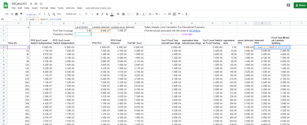
Notice that there is no “if” statement this time, instead we are leveraging a convenient property of the modulo operation: since the modulo operation returns the remainder of division, it’s value oscillates between zero, and the divisor. This is easier to see by example, assume a 1 month (720 hours) proof test frequency:

0mod720 = 0

24mod720 = 24

48mod720 = 48

72mod720 = 72

….

696mod720 = 696

720mod720 = 0

744mod720 = 24

So the modulo expression in our formula bar produces a time which cycles between 0 and 696 (one day before a proof test). Whenever it gets to a time that divides evenly by 720, it conveniently circles back around to 0. Since the PFD at time 0 hours is equal to 0, we don’t even need to do any additional work to incorporate our proof test (because a 100% proof test resets PFD to 0).

Joining the Systems

After both the lambda detected and lambda never detected systems are modeled over the entire mission time (1 yr in our case), all that remains is to combine them. Let’s think through this, do we want to take the intersection of the two systems, or the union?

Well, taking the intersection would imply that we want to know when there is a failure in the lambda never detected system (i.e a failure that we don’t ever find, until we place a demand on the system and it doesn’t work) and there is simultaneously a failure in the lambda detected system (i.e a failure that remains undetected, and will cause our system to not function, until we proof test, at which point we find it and fix it). This isn’t quite right, we don’t need two failures for our system to fail, after all both systems represent the same physical level switch!

A better idea is to take the union of the two systems, this represents the probability that we get either a failure in the never detected system, or a failure in the detected system. If this confuses you, remember that a failure in the lambda detected system still counts as a hidden failure, which will cause our system to not work when a demand is made of it. It’s just that these hidden failures eventually get found and reset to zero at the proof test.

Calculate the union of the two systems based on our familiar formula for unions of two independent events (i.e 2oo2 system). Note that I said independent, we are making an assumption that there is no dependency between the detected and never detected failures: $$\begin{equation} P_A+P_B-P_AP_B \end{equation}$$

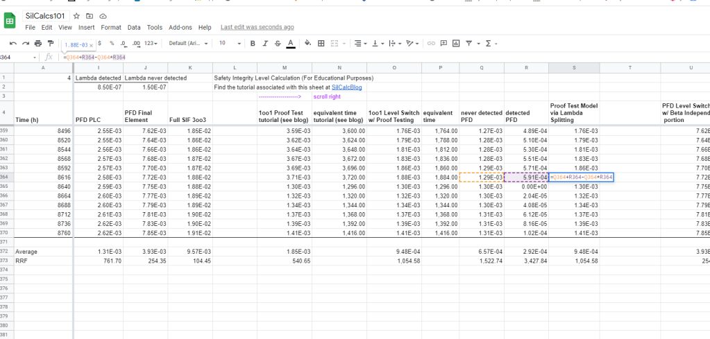
Notice that you get the exact same answer as the method we used above, which I find more intuitive.

Next time, we are going to discuss dependent systems, and common cause failure. Should be a great time.