PFD Equation Derivation

Posted in General on Theoretical

Theoretical post about PFD equation derivation

Edited 17March2023: Improved clarity and fixed typos.

Time for a theoretical post; let’s derive the basic PFD equation we all know and love: $$\begin{equation} PFD = 1 - e^{-\lambda t} \end{equation}$$

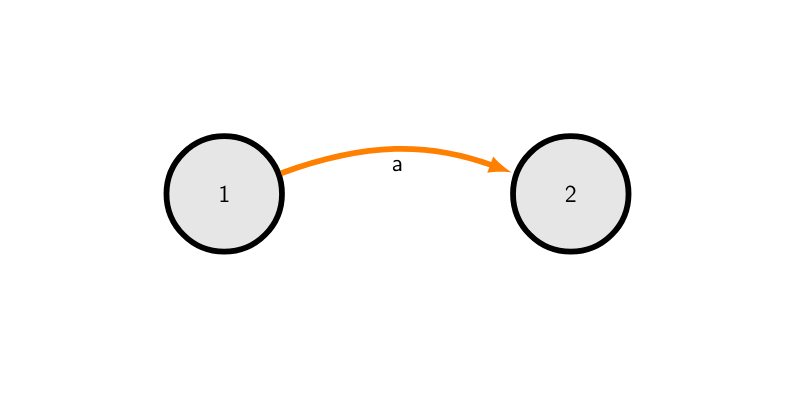
There are a few ways to go about this, but I think the easiest will be to set up a two state system. Consider a system which can either be working, or failed:

Notice that we draw an arc from the working state (state one) to the failed state (state two). Let’s discuss this system a bit; we know that it’s working when we first put it in service (presumably we test it during commissioning). Therefore, we can confidently say that the probability of the system being in state one at time t = 0 is one. We can also assert that the total probability of being in either state one or state two must be unity. Given this info, we can write: $$\begin{align} P_1(0) = 1 \\ P_2(0) = 0 \\ P_1(t) + P_2(t) = 1 \end{align}$$

It will be useful later on to have things in vector form, so lets go ahead and write the probability at time zero in vector form: $$\begin{align} \vec{P}(t) = \biggl[ \begin{array}{c} P_1(t) \\ P_2(t) \end{array} \biggr] \\ \\ \vec{P}(0) = \biggl[ \begin{array}{c} 1 \\ 0 \end{array} \biggr] \end{align}$$

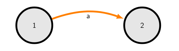
To finish describing the system we need to establish the rate at which we move from state one to state two. For now let’s just call it “a”, and assume that it is constant (i.e. the rate at which we transition from working to failed is not a function of time). “a” has units of 1/time.

Our system now looks like so:

Notice that we are getting dangerously close to a differential equation here. We’ve established that the rate of change from state one to state two, per unit time, is a. If we let the time interval for a approach zero, we have the instantaneous rate at which transitions are made from state one to state two. When multiplied by the probability of being in state one, this gives the rate of change of the probability of being in state one. I.e. : $$\begin{equation} \frac{dP_1}{dt} = -aP_1 \end{equation}$$

Note that P₁ is still a function of time, I have just omitted that for clarity (i.e its P₁(t)).

Also note the negative sign on “a”, this is because “a” is the rate that we are are leaving state one.

We can just solve this equation and be done with the derivation. Solving this equation gives us an expression for P₁, and since P₁+P₂ = 1, we can then quickly solve for P₂, which is what we want (P₂ is the probability, as a function of time, that the system is failed).

The solution is straightforward: notice that this is a first order differential equation, and so we expect the answer to involve an exponential. In words, the above differential equation says “give me a function whose derivative is “-a” times the original function”. We know this will just be an exponential with a factor of “-a” in it: $$\begin{equation} P_1(t) = e^{-at} \end{equation}$$

You can quickly check that this is correct by taking the derivative: $$\begin{equation} \frac{dP_1}{dt} = \frac{d(e^{-at})}{dt}=-ae^{-at}=-aP_1 \end{equation}$$

P₂ is quickly computed: $$\begin{equation} P_2(t) = 1-P_1(t) = 1-e^{-at} \end{equation}$$

And of course, “a” is clearly just our failure rate lambda.

Additional Complications

Before we end this post, lets at least generalize the ideas above a bit.

Notice that if we had more transitions either in or out of state one, then our differential equation would have more terms. In general, we can drop the transition rates into a matrix (coefficient matrix), and use the power of linear algebra to solve the resulting system of differential equations. We’ll cover more complicated systems another time, but for our simple system, with only one transition rate, the matrix looks like this: $$\begin{equation} A =\biggl[\begin{array}{cc} -a&0\\a&0 \end{array}\biggr] \end{equation}$$

Here the matrix position (1,1) represents the total rate at which we are transitioning out of state one. The position (2,1) represents the rate at which we transition to state two from state one. (1,2) represents the rate at which we transition to state one from state two, and (2,2) is the total rate we are transitioning out of state two. Notice that each column sums to zero.

Our system in vector form is then: $$\begin{equation} \frac{d\vec{P}}{dt} = A\vec{P} \end{equation}$$

This is just a system of differential equations, and the solution is an exponential. This time the exponential is raised to the power of a matrix: $$\begin{equation} \vec{P}(t)=e^{At}\vec{P}(0) \end{equation}$$