Simplified Equations: 1oo1 Theory

Posted in Simplified Equations on Theoretical

Theoretical post about simplified Equation equation derivation

• Derivation
• Error Analysis
• Error Is Conservative
• PFD Avg Simplified

Alright, it’s finally time to talk about the simplified equations. In this post, we will start from our familiar basic equation, and discuss how to derive the simplified equation for a 1oo1 system, assuming constant failure rate. The basic idea here is that, as SIS systems get even moderately complex, solving the exact equation for the system’s PFD gets difficult really fast. Recall our previous discussion on multiple element systems, in which we never modeled systems more complex than three elements, and just imagine the pain of doing a real sif by hand! Simplified equations allow you to obtain reasonable answers to real world problems without using fancy commercial software (also, some fancy commercial software uses simplified equations anyway). You can use the equations to get a ballpark estimate on a SIF before doing a more detailed calc, to do a reality check on the aforementioned fancy software, or to actually do your official SIL calcs if you so choose.

Derivation

Derivation of the simplified equations hinges on the properties of the exponential function. Specifically, that the exponential function has a Maclaurin series representation: $$\begin{equation} \sum_{n=0}^{\infty} \frac{x^n}{n!} = 1 + x + \frac{x^2}{2}+\frac{x^3}{6} + ... \end{equation}$$

Substituting -λ*t in for x in the series yields: $$\begin{equation} 1 - \lambda t + \frac{\lambda^2 t^2}{2} - \frac{\lambda^3 t^3}{6} + ... \end{equation}$$

Plugging this series in for the exponential in the PFD equation: $$\begin{align} PFD & = 1 - e^{-\lambda t} = 1 - [1 - \lambda t + \frac{\lambda^2 t^2}{2} - \frac{\lambda^3 t^3}{6} + ...] \\ PFD & = \lambda t - \frac{\lambda^2 t^2}{2} + \frac{\lambda^3 t^3}{6} - ... \end{align}$$

And we have our equation for PFD in the form of an infinite series, which doesn’t seem particularly helpful on first glance. However, we can now experiment with approximating the equation by taking some number of terms (i.e. you can take the first n terms of the series and ask how good of an approximation that is). Specifically, let’s just take the first term, which is alluringly simple: $$\begin{equation} PFD \simeq \lambda t \end{equation}$$

This will be our working approximation for the moment.

Error Analysis

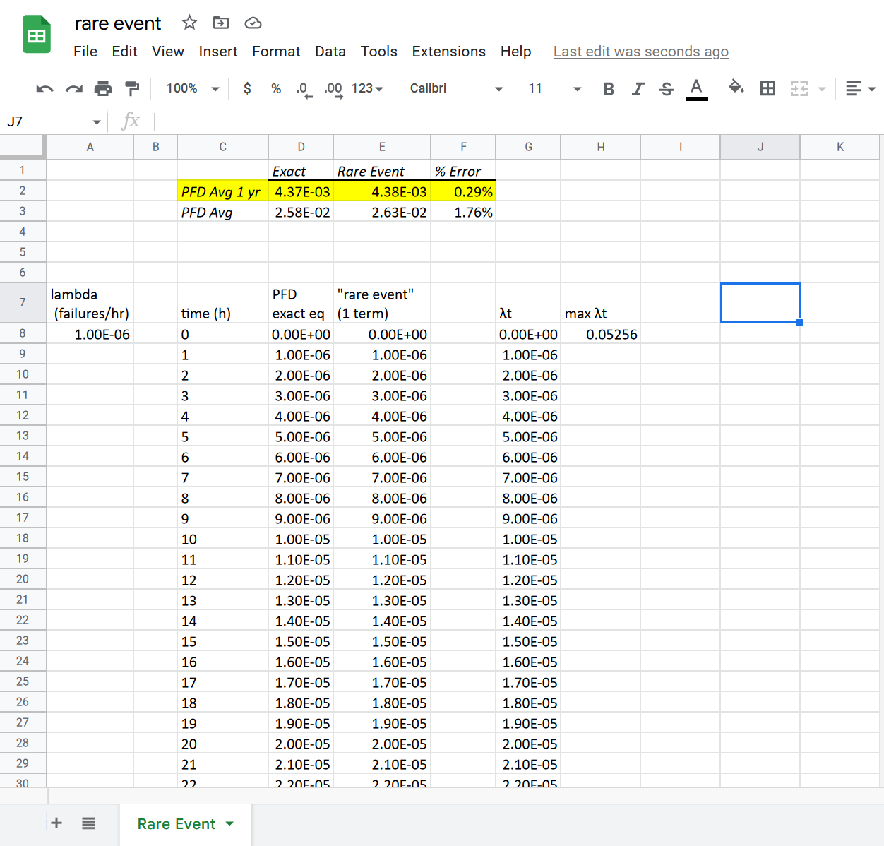
How good of an approximation is this? It would be wonderful if it’s a good one, because such a simple equation is pleasant to work with. Let’s answer this question by doing what we do best around here, model stuff in a spreadsheet. First, we will look at a timeframe of one year, using the failure rate from our trusty level switch. We’ll calculate PFD every hour (similar to how we built the models in SIL Calcs 101, and compare the resulting average PFDs from the exact equation and single term approximation. I am not going to walk through every detail, it’s basically the same procedure as covered in the single element system post. The results are shown below, the error over one year is 0.29%. Notice that the rare event approximation is conservative (i.e. it over estimates the PFD avg), we will see that this is a trend.

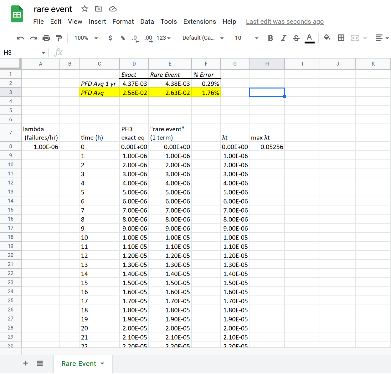
Next, let’s take a look at the error over a six year period. This time we get 1.76% error, and again, the rare event approximation overestimates the PFD avg.

This is typically an acceptable level of error, keep in mind SIL calculations are not meant to be terribly precise, and so only using the first term as the approximation is the typical method. Also, notice that the error is increasing as the timespan increases. In fact, error increases as both timespan, and as lambda increases. To see this, consider a device with a failure rate of 1e-5 (instead of 1e-6):

As you can see, the error over six years jumps up to 18% (still conservative). An important metric to keep an eye on is λt (see columns G and H). ISA-TR84.00.02-2022 recommends limiting λt to 0.1, which limits error in the approximation.

Error Is Conservative

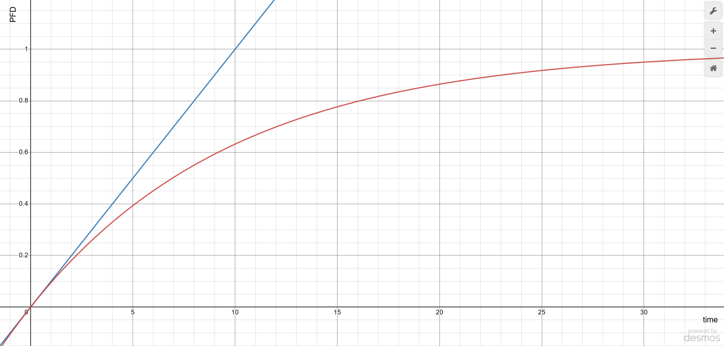
Showing that the error is conservative is relatively straightforward graphically, check out the below plot of the rare event approximation (blue) vs the exact equation (red). Here the y-axis is PFD and the x-axis is time. You can see the the approximation is an upper bound on the exact equation, and thus the approximated PFD will always be higher than the exact PFD.

PFD Avg Simplified

We’ve almost wrapped this post up. The final task is to calculate PFD average now that we have an approximation for PFD. Standard stuff here, calculus tells us that the average of a function over some timeframe is just the integral of the function divided by the timeframe, and the limits of integration correspond to the beginning and end points of the timeframe. It’s probably clearer in symbols than words: $$\begin{equation} PFD_{avg} = \frac{1}{T} \int_{0}^{T} \lambda t \,dt \end{equation}$$

Here “T” is the timeframe over which we want to calculate the PFD Avg. By way of example, above (in the spreadsheet) we were doing this for periods of one year, and six years. Carrying out the integration: $$\begin{align} PFD_{avg} &= \frac{1}{T} \int_{0}^{T} \lambda t \,dt \\ \\ PFD_{avg} &= \frac{1}{T} * \left[\lambda \frac{t^2}{2} \right] _0^T \\ \\ PFD_{avg} &= \frac{1}{T} * \left[\lambda \frac{T^2}{2} \right] \\ \\ PFD_{avg} &= \frac{\lambda T}{2} \end{align}$$

And there you have it, the simplified equation for PFD Avg for a 1oo1 system, under the constant failure rate assumption. We still have more work to do, namely deriving equations for NooM systems, but that will have to wait until next time.